SRP reduction starts from header modifications and correcting for bias. All of these is performed with only text output in terminal. Almost all other routines may plot control graphs during reduction. All of them are also saved into ps files into ps directory.

Cosmic removal

Cosmic removal procedure creates nice FITS files where all detected and (hopefully clearly) removed cosmic rays are marked.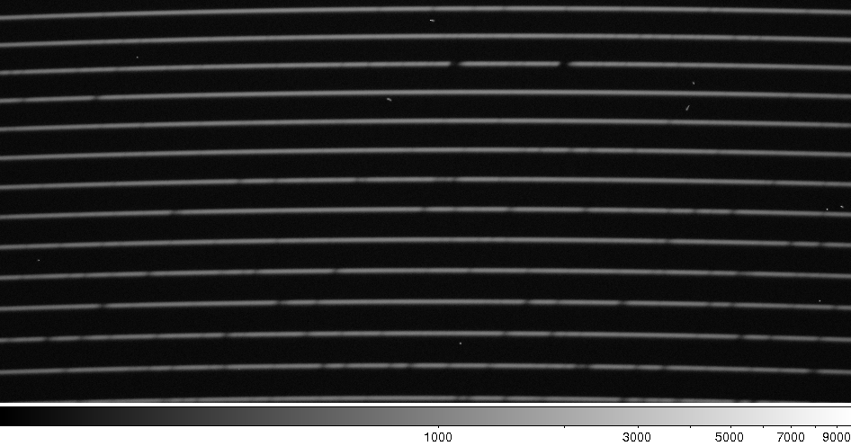

Part of original spectrum after bias reduction.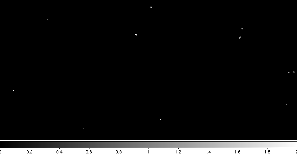

Detected cosmic rays.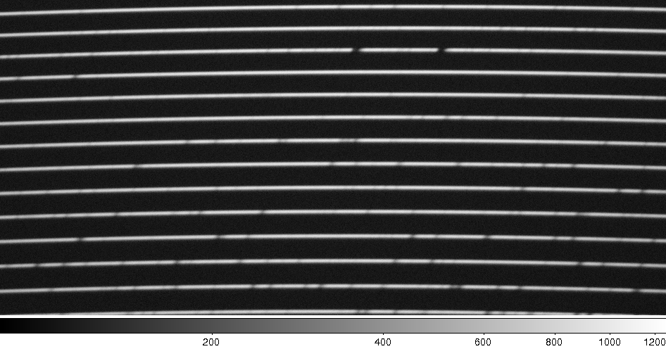

Part of original spectrum after cosmic rays removal.

Tracing

Tracing shows two kind of plots. First with identification of all rows and second with polynomial fitted to each row separately. Additionally a set of pictures (in one ps file) are created, with tracing polynomials over-plotted on traced spectrum.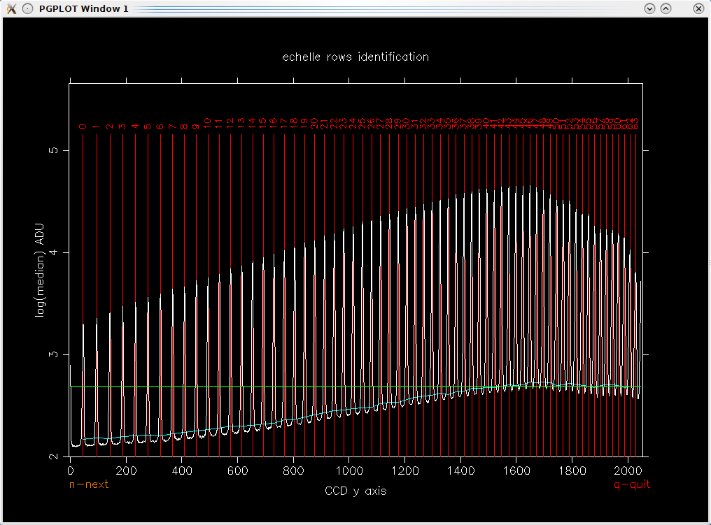

Row identification confirmation plot. This is a median of a vertical, central stripe taken from a spectrum selected for tracing. Background level (blue) and median level (green) are over-plotted.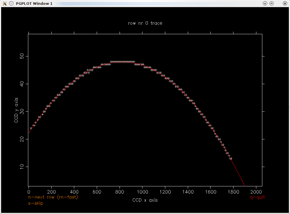

A polynomial fitted to a single row. Each cross is a point estimated to lie in center of that row. Sometimes there are no point at the edges of a row because the signal level is too low to reliably detect it.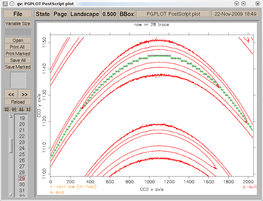

This is a file created by trace procedure that shows an original spectrum (red lines) with trace pints (crosses) and fitted trace function over-plotted.

PSF fitting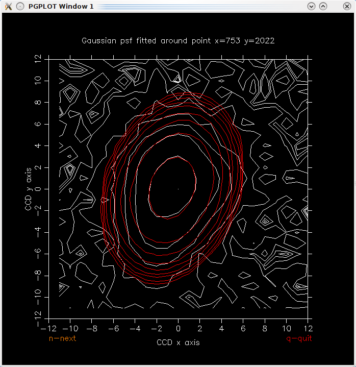

This is a skewed Gaussian fit (red lines) over-plotted on small part of comparison spectrum with selected emission line(white lines).

Extracting 1D spectra

After extracting 1D spectrum SRP is plotting the results for the user to visually verify them.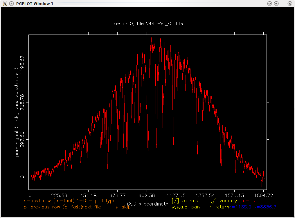

This is a plot of a single row of object spectrum. User can also plot background levels and over-exposition marks.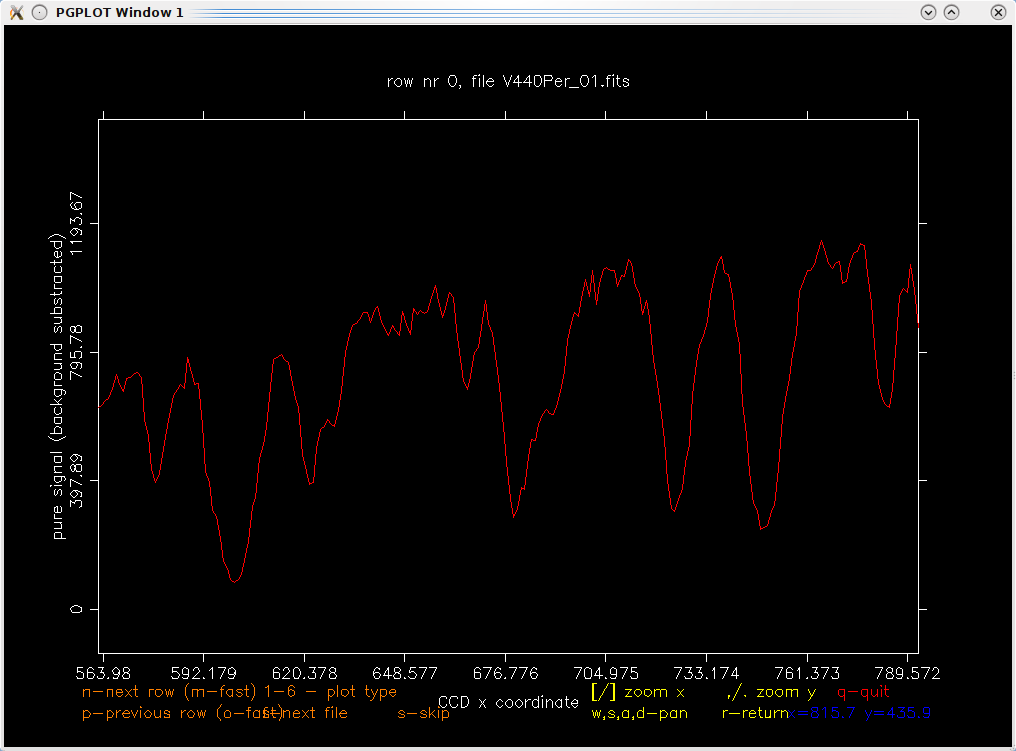

This is just a zoom that shows individual line profiles.

Normalizing master flat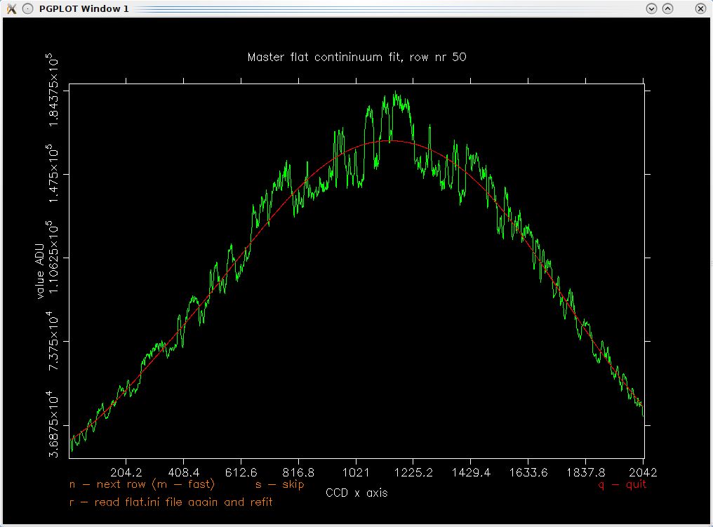

This is a fit of a polynomial to a single row of a master flat spectrum. This row is highly distorted by fringing (we use back-illuminated CCD chip), but a fit seems to be quite good in a center and worse but still acceptable at edges.

Reidentification of comparison spectra

Reidentification of emission lines in comparison spectra can be performed in one or two steps. In the case shown here first a preliminary dispersion model was fitted, than new lines were identified and after that a final model was fitted.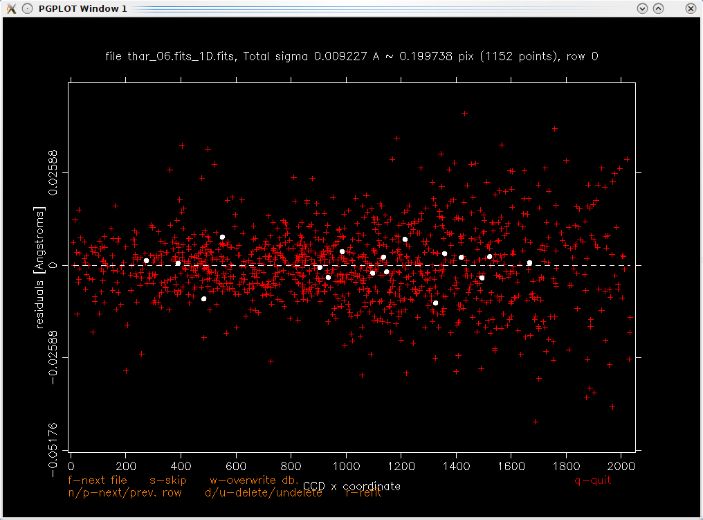

This is a plot with residuals of a preliminary model. They were calculated with weights for row 0 100 times greater than for other rows. Residuals for currently selected row are plotted as white dots.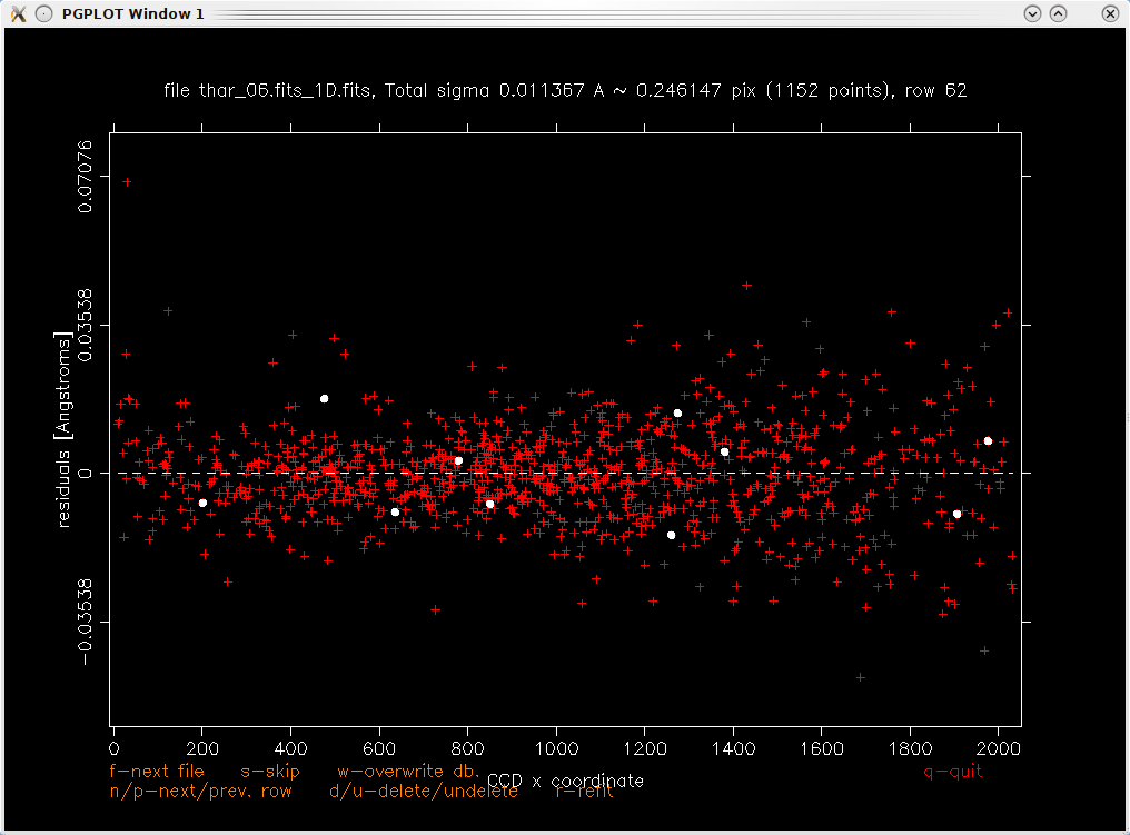

This is a plot with residuals of a preliminary model. This time weights for row 62 were increased. Note that the pattern of residuals changed when comparing with previous plot.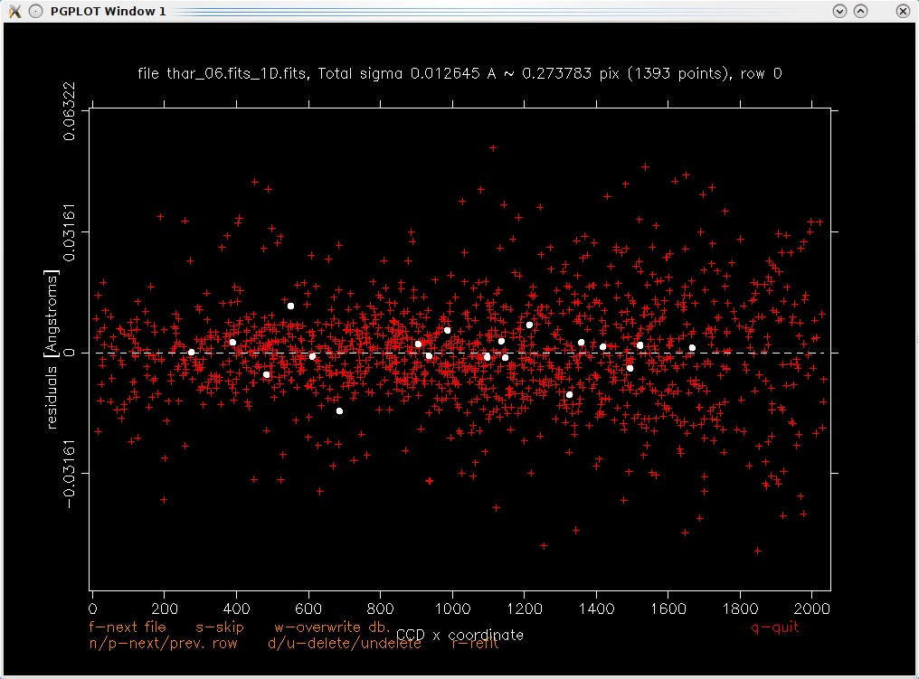

This is a plot with residuals of a final model. Note that the number of identified lines increased from 1152 in previous plots to 1393.

Applying dispersion function

Although applying fitted dispersion function to spectra is automatic it creates nice ps files.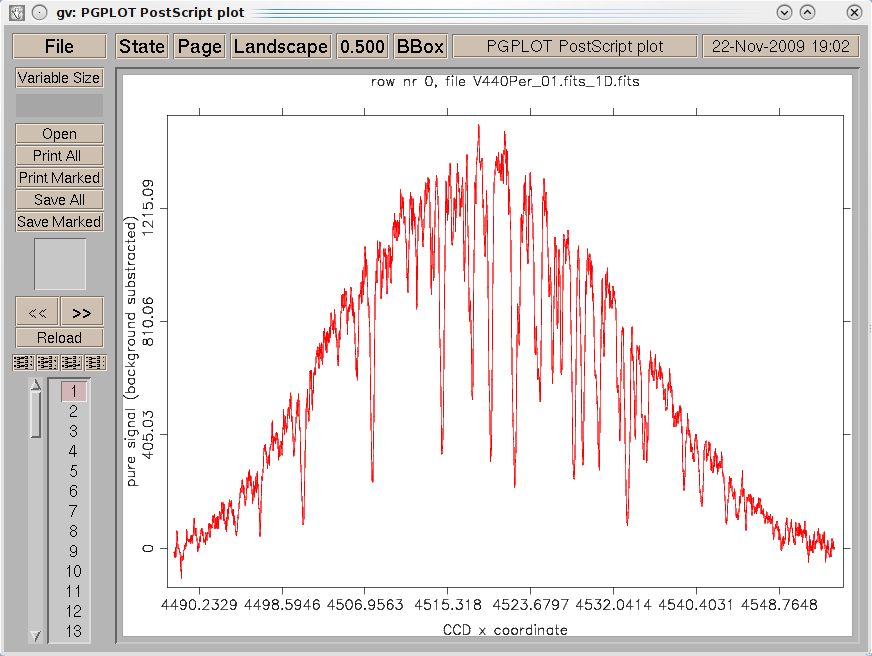

This is a single row from an output ps file created by wav routine. Note that this time you can see wavelengths at the bottom (although there is a mistaken axis name).

Removing continuum

Continuum fitting is also done with graphical output on screen (and simultaneously into ps files).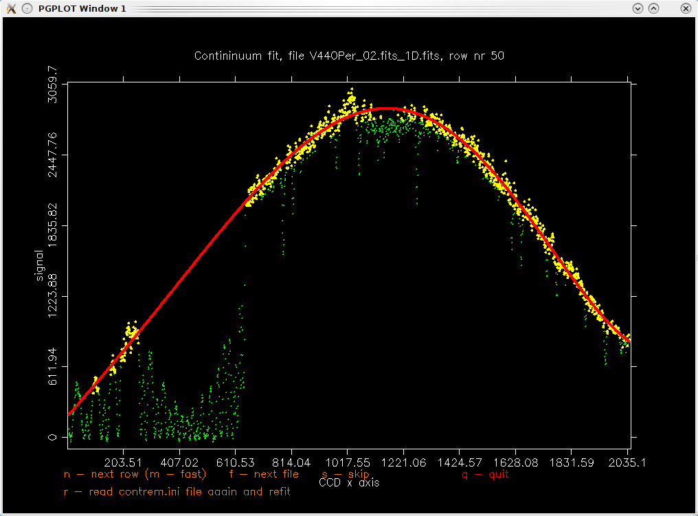

This is an example of continuum fit to a single row of a given spectrum. Too high and too low points are rejected recursively (green points) prior to a final polynomial fit (red line).

Combining all rows

Combination of all rows into a single spectrum is automatic but it outputs the result on screen.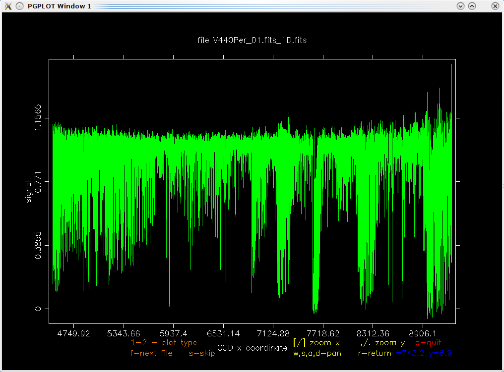

This is an example of a final, resampled and combined spectrum. User can zoom each part and inspect it in details.

Converting to IRAF

Conversion to text files that are easy to import to IRAF is done without any graphical output. Nevertheless one can plot spectra after importing to IRAF with eg. splot routine.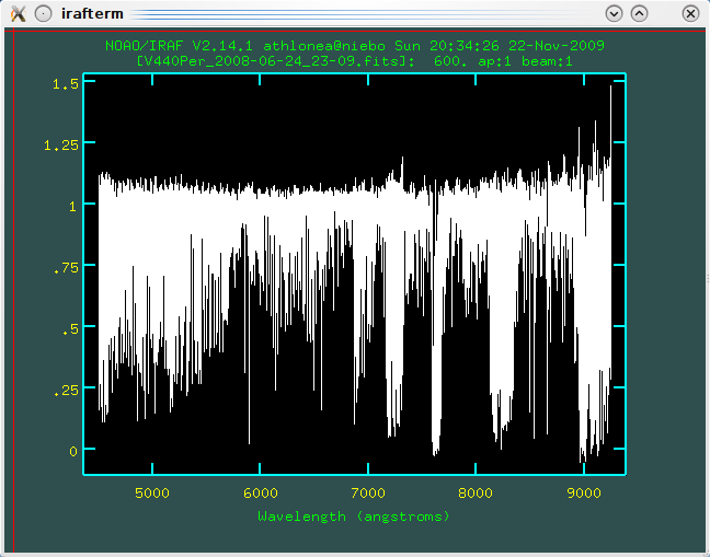

Spectrum reduced by SRP that has been imported to IRAF. This plot was created with splot routine.